Histogram Equalization in Digital Image Processing
A beginner-friendly introduction to histogram equalization and image contrast enhancement
Catalog
Click on this table of contents to jump to the corresponding section
A digital image is a two-dimensional matrix of two spatial coordinates, with each cell specifying the intensity level of the image at that point. So, we have an N x N matrix with integer values ranging from a minimum intensity level of 0 to a maximum level of L-1, where L denotes the number of intensity levels. Hence, the intensity levels of a pixel r can take on values from 0,1,2,3,.... (L-1). Generally, L = [@portabletext/react] Unknown block type "latex", specify a component for it in the `components.types` prop, where m is the number of bits required to represent the intensity levels. Zero level intensity denotes complete black or dark, whereas L-1 level indicates complete white or absence of grayscale.
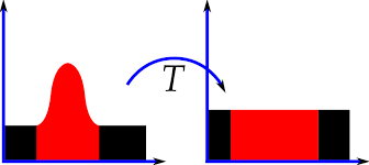
Intensity Transformation:
Intensity transformation is a basic digital image processing technique, where the pixel intensity levels of an image are transformed to new values using a mathematical transformation function, so as to get a new output image. In essence, intensity transformations is simply to implement the following function:
where s is the new pixel intensity level and r is the original pixel intensity value of the given image and r≥0.
With different forms of the transformation function T(r), we get different output images.
Common Intensity Transformation Functions:
1. Image negation: This reverses the grayscales of an image, making dark pixels whiter and white pixels darker. This is completely analogous to the photographic negative, hence the name.
2. Log Transform: Here c is some constant. It is used for expanding the dark pixel values in an image.
3. Power-law Transform: Here c and γ are some arbitrary constants. This transform can be used for a variety of purposes by varying the value of γ.
Histogram Equalization:
The histogram of digital image, with intensity levels between 0 and (L-1), is a function [@portabletext/react] Unknown block type "latex", specify a component for it in the `components.types` prop, where [@portabletext/react] Unknown block type "latex", specify a component for it in the `components.types` propis [@portabletext/react] Unknown block type "latex", specify a component for it in the `components.types` prop intensity and [@portabletext/react] Unknown block type "latex", specify a component for it in the `components.types` propis the number of pixels in the image haivng that intensity levels. We can also normalize the histogram by dividing it by the total number of pixels in the image. For an NxN image, we have the following definition of normalized histogram function:
This [@portabletext/react] Unknown block type "latex", specify a component for it in the `components.types` prop function is the probability of the occurrence of a pixel with the intensity level [@portabletext/react] Unknown block type "latex", specify a component for it in the `components.types` prop . Clearly
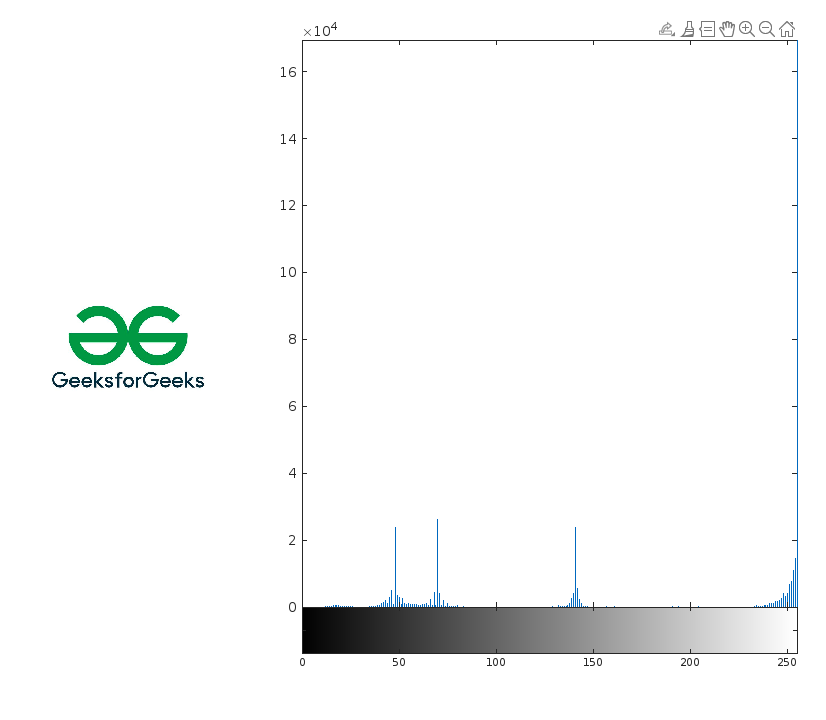
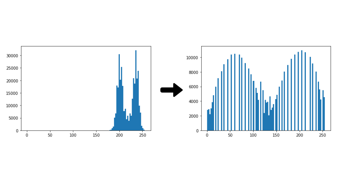
The histogram of an image, as shown in the figure, consists of the x-axis representing the intensity levels [@portabletext/react] Unknown block type "latex", specify a component for it in the `components.types` prop and the y-axis denoting the [@portabletext/react] Unknown block type "latex", specify a component for it in the `components.types` prop or the [@portabletext/react] Unknown block type "latex", specify a component for it in the `components.types` prop functions.
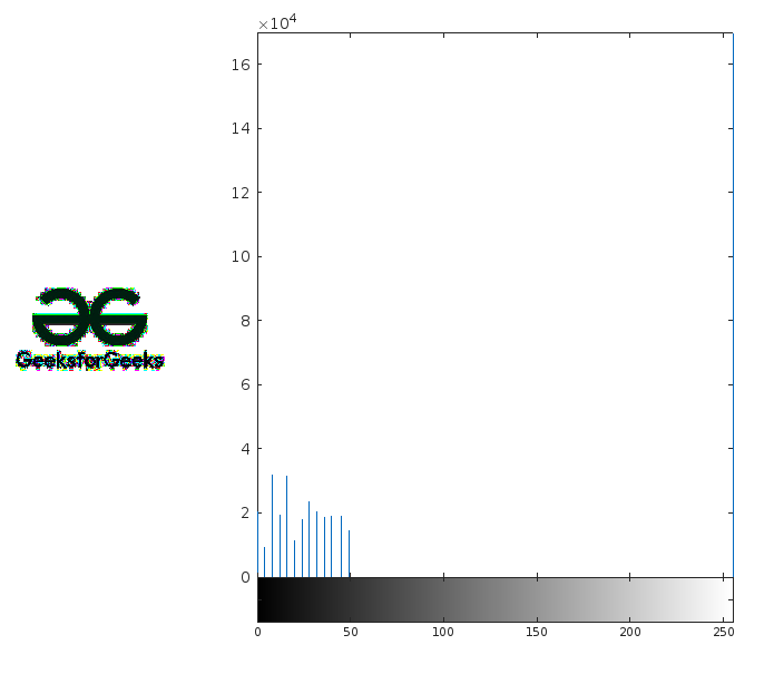
The histogram of an image gives important information about the grayscale and contrast of the image. If the entire histogram of an image is centered towards the left end of the x-axis, then it implies a dark image. If the histogram is more inclined towards the right end, it signifies a white or bright image. A narrow-width histogram plot at the center of the intensity axis shows a low-contrast image, as it has a few levels of grayscale. On the other hand, an evenly distributed histogram over the entire x-axis gives a high-contrast effect to the image.
In image processing, there frequently arises the need to improve the contrast of the image. In such cases, we use an intensity transformation technique known as histogram equalization. Histogram equalization is the process of uniformly distributing the image histogram over the entire intensity axis by choosing a proper intensity transformation function. Hence, histogram equalization is an intensity transformation process.
The choice of the ideal transformation function for uniform distribution of the image histogram is mathematically explained below.
Mathematical Derivation of Transformation Function for Histogram Equalization:
Let us consider that the intensity levels of the image r is continuous, unlike the discrete case in digital images. We limit the values that r can take between 0 and L-1, that is, 0 ≤ r ≤ L-1 . r = 0 represents black and r = L-1 represents white. Let us consider an arbitrary transformation function:
where s denotes the intensity levels of the resultant image. We have certain constraints on T(r).
- T(r) must be a strictly increasing function. This makes it an injective function.
- 0 ≤ T( r ) ≤ L-1. This makes T(r) surjective.
The above two conditions make T(r) a bijective function. We know that such functions are invertible. So we can get back r values from s. We can have a function such that [@portabletext/react] Unknown block type "latex", specify a component for it in the `components.types` prop
Let us now say that the probability density function (pdf) of r is [@portabletext/react] Unknown block type "latex", specify a component for it in the `components.types` propand the cumulative distribution function (CDF) of r is [@portabletext/react] Unknown block type "latex", specify a component for it in the `components.types` prop. Now the CDF of s will be:
We put the first condition of T(r) precisely to make the above step hold true. The second condition is needed as s is the intensity value for the output image and so must be between 0 and (L-1).
So, a pdf of s can be obtained by differentiating [@portabletext/react] Unknown block type "latex", specify a component for it in the `components.types` propwith respect to x. We get the following relation:
Now, if we define the transformation function as follows:
Then using this function gives us a uniform pdf for s.
The above step used Leibnitz's integral rule. Using the above derivative, we get:
So the pdf of s is uniform. This is what we want.
Now, we extend the above continuous case to the discrete case. The natural replacement of the integral sign is the summation. Hence, we are left with the following histogram equalization transformation function.
Since s must have integer values, any non-integer value obtained from the above function is rounded off to the nearest integer.
Example 1:
Output:
Example 2:
Lily and 4 people like this

Prev Post
Space The Final Frontier
Next Post
Telescopes 101

0 Comments
Leave a Reply
Recent Post
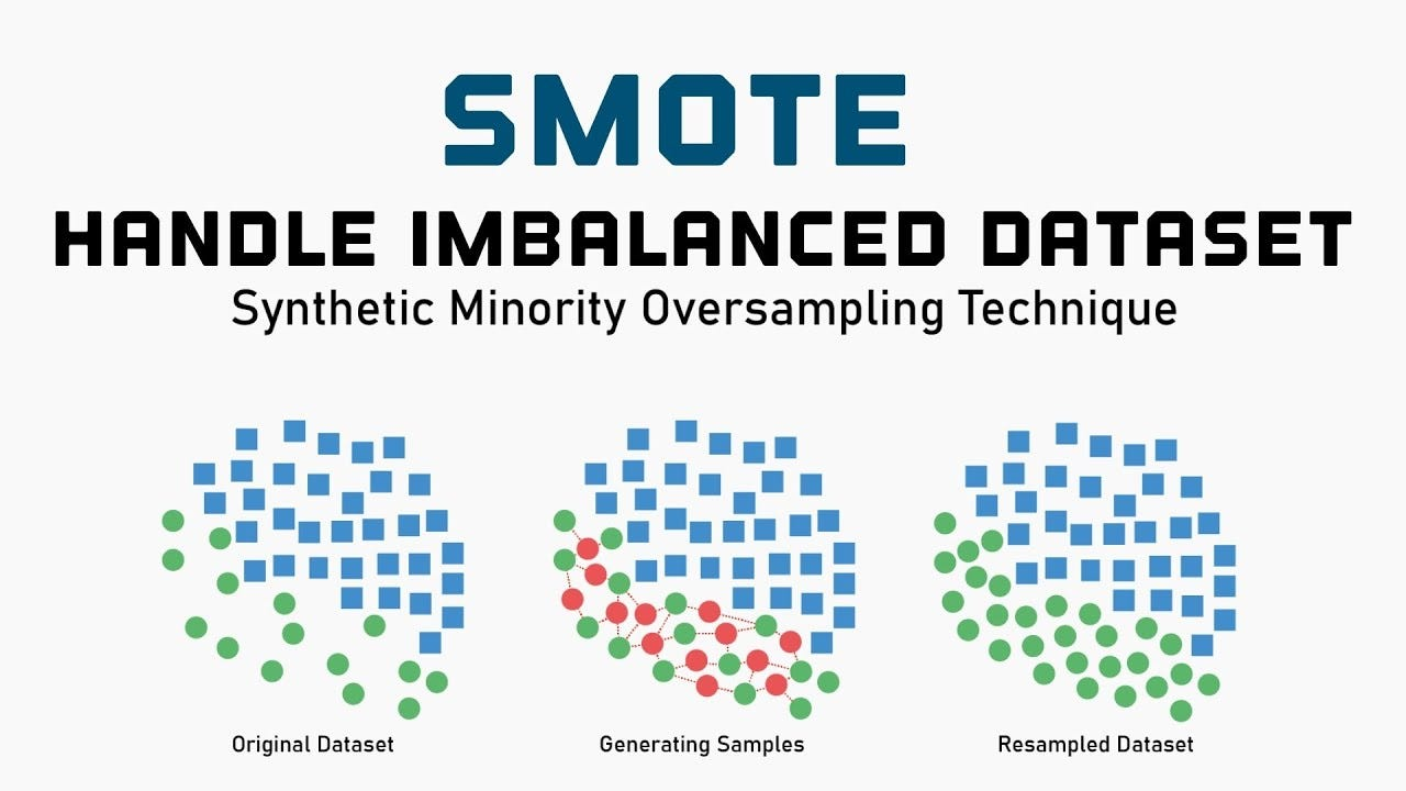
SMOTE for Imbalanced Classification with Python
12:28:00 16/05/2026
CLAHE Histogram Equalization with OpenCV: A Python Guide
12:06:00 16/05/2026
Histogram Equalization in Digital Image Processing
10:56:00 16/05/2026
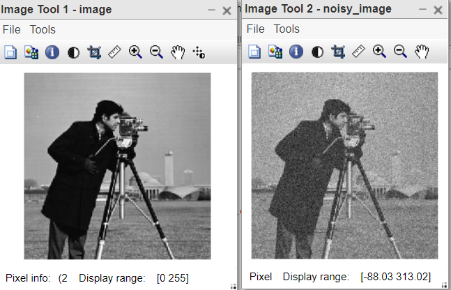
Gaussian Noise Explained: What It Is and How It Works
10:36:00 16/05/2026
Python Image Blurring with OpenCV: Gaussian, Median & Bilateral Filter Guide
09:59:00 16/05/2026
Related Topics
Feeds
Don't miss what's next 👋
Enjoyed this content? Leave your email to get notified when we publish new insights, tutorials, and updates — no spam, ever.