SIFT Interest Point Detector Using Python and OpenCV: A Complete Step-by-Step Guide

SIFT (Scale Invariant Feature Transform) Dectector is used in the detections of interest points on an input image. It allows the identification of localized features in images which essential in applications such as:

• Object Recognition in Images
• Path detection and obstacle avoidance algorithms
• Gesture recognition, Mosaic generation, etc.

Unlike the Harris Detector, which is dependent on properties of the image such as viewpoint, depth, and scale. SIFT can perform feature detection independent of these properties of the image. This is achieved by the transformation of the image data into scale-invariant coordinates. The SIFT Detector has been said to be a close approximation of the system used in the primate visual system.

Steps for Extracting Interest Points

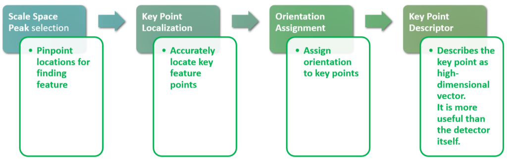
Phase I: Scale Space Peak Selection

The concept of Scale Space deals with the application of a continous range of Gaussin Filters to the target image such that the chosen Gaussian have differing values of the sigma parameter. The plot thus obtained is called the Scale Space. Scale Space Peak Selections depends on the Spatial Coincidence Assumption.

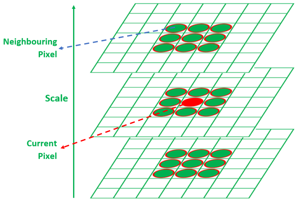
In 2D images, we can detect the Interest Points using the local maxima/minima in Scale Space of Laplacian of Gaussian. A potential SIFT interest point is determined for a given sigma value by picking the potential interest point and considering the pixels in the level above (with higher sigma), the same level, and the level below (with lower sigma than current sigma level). If the point is maxima/minima of all these 26 neighboring points. It is a potential SIFT interest point - and it acts as a starting point for interest point detection.

Phase II: Key Point Localization

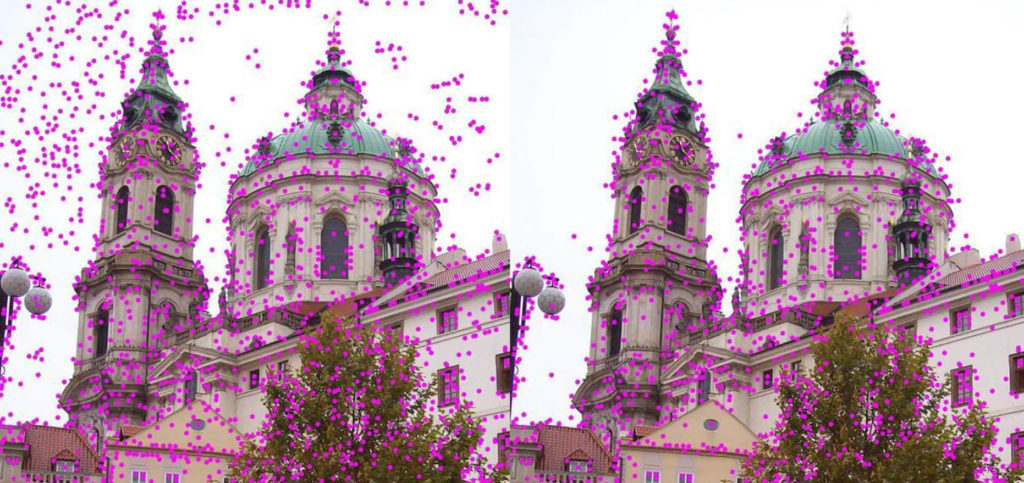
Key point localization involves the refinement of keypoints selected in the previous stage. Low constast key-points, unstable key points, and keypoints lying on edges are eliminated. This is achieved by calculating the Laplacian of the keypoints found in the previous stage. The extrema values are computed as follows:

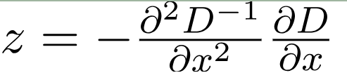
In the above expression, D represents the Difference of Gaussian. To remove the unstable key points, the value of z is calculated and if the function value at z is below a threshold value then the point is excluded.

Phase III: Assigning Orientation to Keypoints

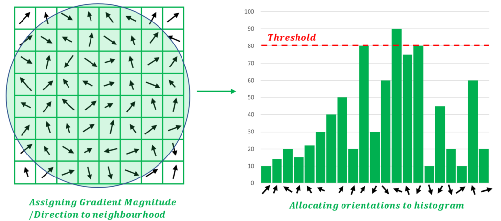
To achieve detection which is invariant with respect the rotation of the image, orientation needs to be calculated for the key-points. This is done by considering the neighborhood of the keypoint and calculating the magnitude and direction of gradients of the neighborhood. Based on the values obtained, a histogram is constructured with 36 bins to represent 360 degrees of orientation (10 degrees per bin). Thus, if the gradient direction of a certain point is say, 67.8 degrees, a value, proportional to the gradient magnitude of this point, is added to the bin representing 60-70 degrees. Histogram peaks above 80% are converted into a new keypoint are used to decide the orientation of the original keypoint.

Phase IV: Key Point Descriptor

Finally, for each keypoint, a descriptor is created using the keypoints neightborhood. These descriptors are used for matching keypoints across images. A 16x16 neighborhood of the keypoint is used for defining the descriptor of that key-point. This 16x15 neighborhood is divided into sub-block. Each such sub-block is a non-overlapping, contiguous, 4x4 neighborhood. Subsequently, for each sub-block, an 8 bin orientation is created similarly as discussed in Orientation Assignment. These 128 bin values (16 sub-blocks * 8 bins per block) are represented as a vector to generate the keypoint descriptor.

Example: SIFT detector in Python

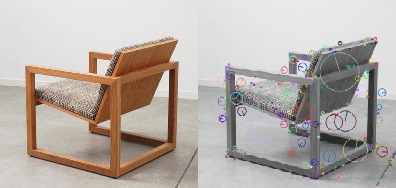
Running the following script in the same directory with a file named "geeks.jpg" generates the "image-with-keypoints.jpg" which contains the interest points, detected using the SIFT module in OpenCV, marked using circular overlays.

Below is the implementation:

# Important NOTE:  Use opencv >=4.4 
import cv2

# Loading the image
img = cv2.imread('geeks.jpg')

 # Converting image to grayscale
gray= cv2.cvtColor(img,cv2.COLOR_BGR2GRAY)

# Applying SIFT detector
sift = cv.SIFT_create()
kp = sift.detect(gray, None)

# Marking the keypoint on the image using circles
img=cv2.drawKeypoints(gray ,
                      kp ,
                      img ,
                      flags=cv2.DRAW_MATCHES_FLAGS_DRAW_RICH_KEYPOINTS)

cv2.imwrite('image-with-keypoints.jpg', img)

Output: