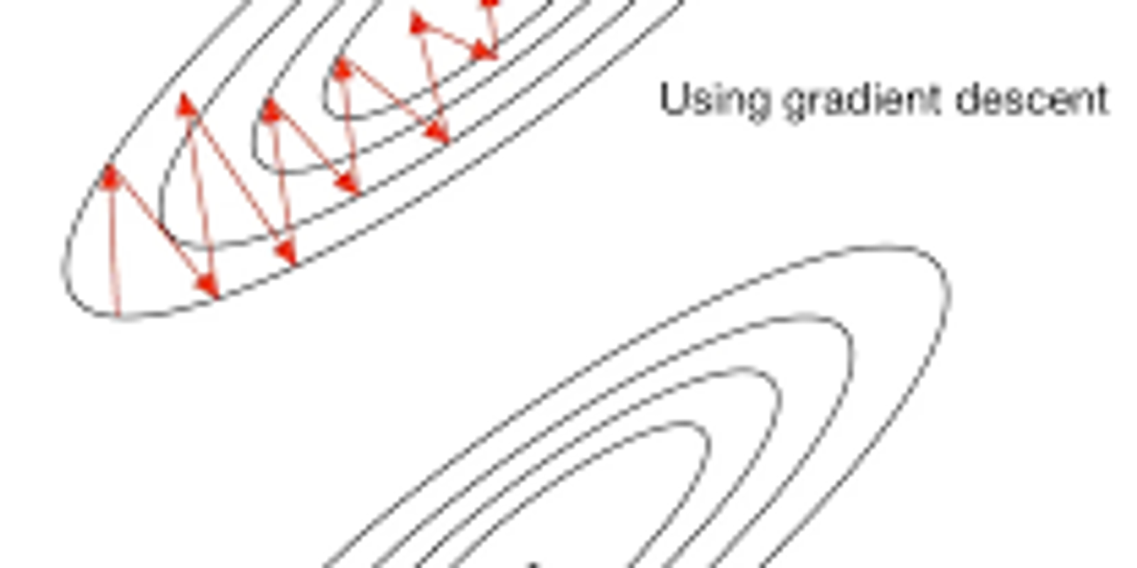
RMSProp Optimizer – Adaptive Learning Rate for Deep Learning

RMSProp (Root Mean Square Propagation) is an adaptive learning rate optimization algorithm designed to improve the performance and speed of training deep learning models.

• It is a variant of the gradient descent algorithm which adapts the learning rate for each parameter individually by considering the magnitude of recent gradients for those parameters.
• This adaptive nature helps in dealing with the challenges of non-stationary objectives and sparse gradients commonly encountered in deep learning tasks.

Need of RMSProp Optimizer

RMSProp was developed to address the limitations of previous optimization methods such as SGD (Stochastic Gradient Descent) and AdaGrad as SGD uses a constant learning rate which can be inefficient and AdaGrad reduces the learning rate too aggressively.

RMSProp balances by adapting the learning rates based on a moving average of squared gradients. This approach helps in maintaining a balance between efficient convergence and stability during the training process making RMSProp a widely used optimization algorithm in modern deep learning.

How RMSProp Works?

RMSProp keeps a moving average of the squared gradients to normalize the gradient updates. By doing so it prevents the learning rate from becoming too small which was a drawback in AdaGrad and ensures that the updates are appropriately scaled for each parameter. This mechanism allows RMSProp to perform well event in the presence of non-stationary objectives making it suitable for training deep learning models.

The mathematical formulation is as follows:

1. Compute the gradient [@portabletext/react] Unknown block type "latex", specify a component for it in the `components.types` prop at time step t:

2. Update the moving average of squared gradients:

where γ is the decay rate.

3. Update the parameter θθ using the adjusted learning rate:

​where η is the learning rate and ϵϵ is a small constant added for numerical stability.

Parameters Used in RMSProp

• Learning Rate (ηη): Controls the step size during the parameter updates. RMSProp typically uses a default learning rate of 0.001, but it can be adjusted based on the specific problem.
• Decay Rate (γγ): Determines how quickly the moving average of squared gradients decays. A common default value is 0.9 which balances the contribution of recent and past gradients.
• Epsilon (ϵϵ): A small constant added to the denominator to prevent division by zero and ensure numerical stability. A typical value for ϵϵ is 1e-8.

By carefully adjusting these parameters, RMSProp effectively adapts the learning rates during training, leading to faster and more reliable convergence in deep learning models.

Implementing RMSprop in Python using TensorFlow or Keras

We will use the following code line for initializing the RMSProp optimizer with hyperparameters:

tf.keras.optimizers.RMSprop(learning_rate=0.001, rho=0.9)

• learning_rate=0.001: Sets the step size for weight updates. Smaller learning rates result in smaller updates, helping to fine-tune weights and prevent overshooting the minimum loss.
• rho=0.9: The discounting factor for the history of gradients, controlling the influence of past gradients on the current gradient computation.

1. Importing Libraries

We are importing libraries to implement RMSprop optimizer, handle datasets, build the model and plot results.

• tensorflow.keras for deep learning components.
• matplotlib.pyplot for visualization.

import tensorflow as tf
from tensorflow.keras.datasets import mnist
from tensorflow.keras.models import Sequential
from tensorflow.keras.layers import Dense, Flatten
from tensorflow.keras.utils import to_categorical
import matplotlib.pyplot as plt

2. Loading and Preprocessing Dataset

We load the MNIST dataset, normalize pixel values to [0,1] and one-hot encode labels.

• mnist.load_data() loads images and labels.
• Normalization improves training stability.
• to_categorical() converts labels to one-hot vectors.

(x_train, y_train), (x_test, y_test) = mnist.load_data()

x_train = x_train.astype('float32') / 255.0
x_test = x_test.astype('float32') / 255.0
y_train = to_categorical(y_train, 10)
y_test = to_categorical(y_test, 10)

3. Building the Model

We define a neural network using Sequential with input flattening and dense layers.

• Flatten converts 2D images to 1D vectors.
• Dense layers learn pattens with ReLU and softmax activations.

model = Sequential([
    Flatten(input_shape=(28, 28)),
    Dense(128, activation='relu'),
    Dense(64, activation='relu'),
    Dense(10, activation='softmax')
])

4. Compiling the Model

We compile the model using the RMSprop optimizer for adaptive learning rates, categorical cross-entropy loss for multi-class classification and track accuracy metric.

• RMSprop adjusts learning rates based on recent gradients (parameter rho controls decay rate).
• categorical_crossentropy suits one-hot encoded labels.

model.compile(optimizer=tf.keras.optimizers.RMSprop(learning_rate=0.001, rho=0.9),
              loss='categorical_crossentropy',
              metrics=['accuracy'])

5. Training the Model

We train the model over 10 epochs with batch size 32 and validate on 20% of training data. validation_split monitors model performance on unseen data each epoch.

history = model.fit(x_train, y_train, epochs=10,
                    batch_size=32, validation_split=0.2)

6. Evaluating and Visualizing Results

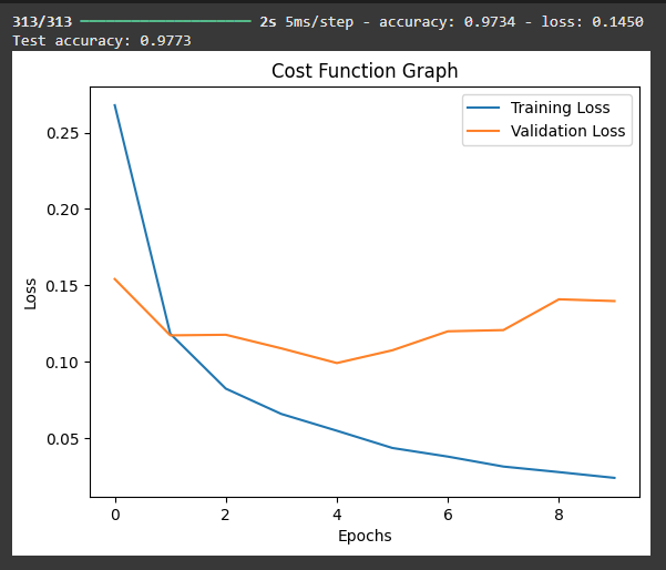
We evaluate test accuracy on unseen test data and plot training and validation loss curves to visualize learning progress.

loss, accuracy = model.evaluate(x_test, y_test)
print(f'Test accuracy: {accuracy:.4f}')

plt.plot(history.history['loss'], label='Training Loss')
plt.plot(history.history['val_loss'], label='Validation Loss')
plt.xlabel('Epochs')
plt.ylabel('Loss')
plt.title('Cost Function Graph')
plt.legend()
plt.show()

Advantages

• Adaptive Learning Rates: Adjusts learning rates for each parameter individually, optimizing updates more effectively.
• Handles Non-Stationary Objectives: Efficiently adapts to changing optimal parameter values over time.
• Prevents Learning Rate Decay Problem: Maintains optimal learning rates by using a decay rate unlike AdaGrad.
• Improved Convergence Speed: Faster convergence due to balanced and dynamic learning rates.

Disadvantages

• Sensitivity to Hyperparameters: Performance is sensitive to settings like decay rate and epsilon meaning it requires careful tuning.
• Poor Performance with Sparse Data: May struggle with sparse data, leading to slower or inconsistent convergence.