ResNet Explained: Solving Deep Neural Network Problems with Residual Learning

To overcome the challenges of training very deep neural networks. Residual Networks (ResNet) was introduced, which uses skip connections that allow the model to learn residual mappings instead of direct transformations make deep neural networks easier to train

• It helps prevent vanishing gradient problems in very deep models.
• Skip connections let information flow directly across layers
• ResNet enables building networks with hundreds or even thousands of layers.
• It is widely used in computer vision tasks like image classification and object detection

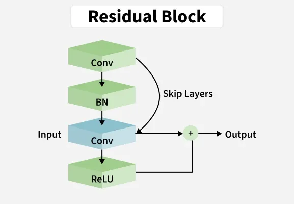
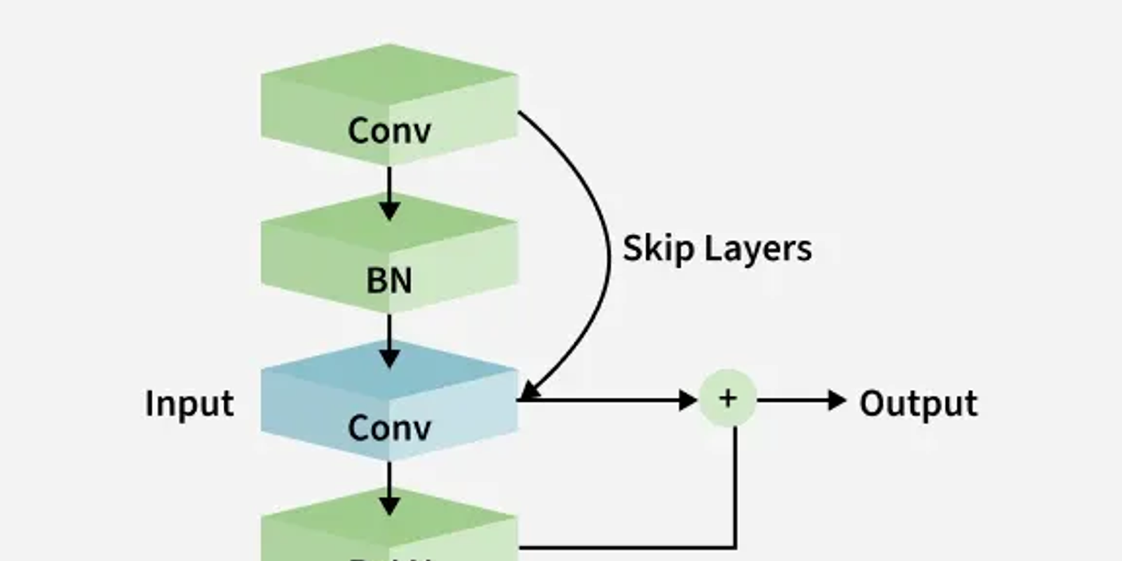
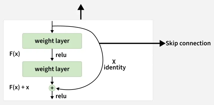
A residual block lets the network skip layers by adding the original input to the processed output, making deep networks easier to train.

Challenges in Deep Neural Networks

Deep Neural Networks are useful models but they also come with several traning challenges, especially as the network depth increases.

Two major issues are

1. Vanishing/Exploding Gradient Problem: As the number of layers in a neural network increases, the gradients of the loss function with respect to the weights can become extremely small or excessively large during backpropagation.

2. Degradation Problem: The degradation problem occurs when increasing the network depth does not improve performance and may even worsen it. This problem has two aspects:

• Performance Plateau: Training error saturates after a certain depth meaning additional layers do not significantly reduce the error.
• Accuracy Degradation: Beyond a certain depth validation error increases and the model performs poorly on unseen data.

Understanding ResNet

ResNet is a deep learning architecture designed to train very deep networks efficiently using residual connections. Here are the key features of ResNet:

• Residual Connections: Enable very deep networks by allowing gradients to flow through identity shortcuts, reducing the vanishing gradient problem.
• Identity Mapping: Simplifies training by learning residual functions instead of full mappings.
• Depth: Supports extremely deep architectures for improved image recognition performance.
• Fewer Parameters: Achieves high accuracy with fewer parameters hence improving computational efficiency.
• Results: Delivers top performance on benchmark image recognition tasks.
• Effective Approach: Residual connections provide a reliable way to train deeper networks effectively, enabling networks to learn mode complex features.

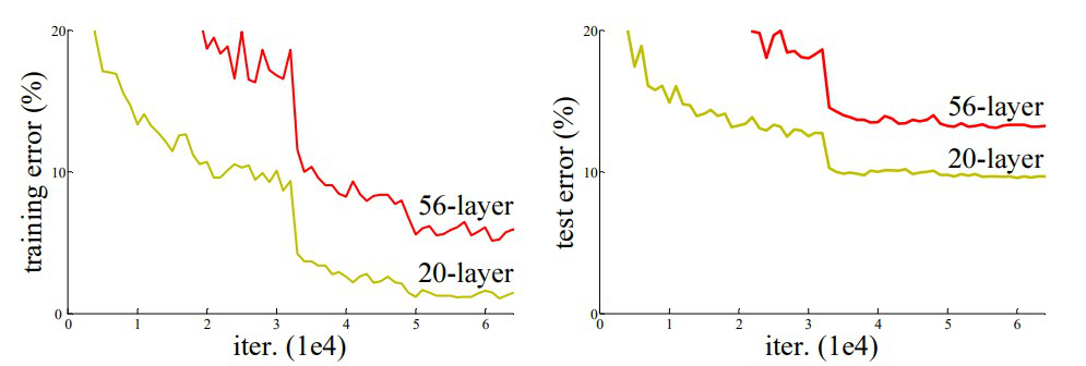
• Left graph (training error): The 56 layer network reduces error slowly and shows strong fluctuations due to vanishing gradients, whereas the 20-layer network learns smoothly and reaches a much lower training error.
• Right graph (test error): The 56-layer network maintains a higher test error (degradation problem), while the 20-layer network generalizes better showing why ResNet skip connections are essential for training deep models.

ResNet-34

ResNet-34 is a deep residual network built on a 34-layer plain network inspired by VGG-19, with shortcut connections forming 16 residual blocks.

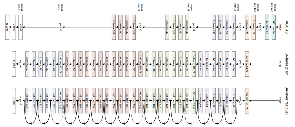
Here are the different stages of the ResNet-34 architecture, showing its structured arrangement of residual blocks.

• First set: 3 residual blocks each with 2 convolution layers of 64 filters and identity skip connections.
• Second set: 4 residual blocks each with 2 convolution layers of 128 filters uses zero-padding or 1x1 projections for dimension changes.
• Third set: 6 residual blocks, each with 2 convolution layers of 256 filters.
• Fourth set: 3 residual blocks with 2 convolution layers of 512 filters each.
• Feature map: Passed through Global Average Pooling a dense layer with 1000 neurons and softmax for classification.

How ResNet Works

Conventional networks try to learn the full mapping H(x)H(x). ResNet instead learns a residual function and combines it with the input via a skip connection.

H(x)=F(x)+x

where:

• x: input to the block
• H(x): desired mapping
• F(x): residual function to be learned

Learning the simpler residual F(x) makes optimization easier.

1. Residual Block: A Residual Block contains:

• One or more convolutional layers
• A skip connection that bypasses these layers
• Addition of input to convolution output
• This ensures uninterrupted flow of information and gradients

2. Skip (Shortcut) Connection

• Bypasses one or more layers
• Adds input directly to output
• Prevents vanishing gradients
• Improves parameter updates

3. Handling Dimension Mismatch: When input and output dimensions differ

• Zero Padding: Adds extra zeros to the input to match output dimensions in a residual block
• Linear Projection: Uses a learnable 1x1 convolution to match input and output dimensions for the skip connection.

3. Stacking Residual Blocks : Multiple residual blocks can be stacked to create deep architectures. This allows networks to go very deep without suffering from degradation.

4. Global Average Pooling (GAP): Before the final fully connected layer ResNet uses GAP:

• Converts each feature map to a single value by averaging
• Reduces parameters less overfitting
• Produces compact feature representation

Step-By-Step Implementation

Here we implement ResNet (v1 and v2) for CIFAR-10. We will cover data preprocessing, model creation, training and plotting graphs step by step.

Step 1: Import Libraries

import tensorflow as tf
from tensorflow import keras
from tensorflow.keras.layers import Dense, Conv2D, BatchNormalization, Activation
from tensorflow.keras.layers import AveragePooling2D, Input, Flatten, Add
from tensorflow.keras.optimizers import Adam
from tensorflow.keras.callbacks import ModelCheckpoint, LearningRateScheduler, ReduceLROnPlateau
from tensorflow.keras.preprocessing.image import ImageDataGenerator
from tensorflow.keras.regularizers import l2
from tensorflow.keras.models import Model
from tensorflow.keras.datasets import cifar10
import numpy as np
import os

Step 2: Set Hyperparameters

• Set batch_size, epochs, num_classes and data_augmentation
• Choose ResNet version and number of residual blocks
• Compute depth based on CIFAR ResNet rules

batch_size = 32
epochs = 200
data_augmentation = True
num_classes = 10
subtract_pixel_mean = True
n = 3
version = 1  

if version == 1:
    depth = n * 6 + 2
elif version == 2:
    depth = n * 9 + 2

model_type = 'ResNet %dv%d' % (depth, version)

Step 3: Load and Preprocess CIFAR-10 Data

• Load CIFAR-10 dataset using Keras.
• Normalize pixel values to range [0, 1].
• Optionally subtract the dataset mean for zero-centered input.
• Convert labels to one hot vectors.

(x_train, y_train), (x_test, y_test) = cifar10.load_data()
input_shape = x_train.shape[1:]


x_train = x_train.astype('float32') / 255
x_test = x_test.astype('float32') / 255

if subtract_pixel_mean:
    x_train_mean = np.mean(x_train, axis=0)
    x_train -= x_train_mean
    x_test -= x_train_mean

y_train = keras.utils.to_categorical(y_train, num_classes)
y_test = keras.utils.to_categorical(y_test, num_classes)

print('x_train shape:', x_train.shape)
print('y_train shape:', y_train.shape)

Step 4: Defining Learning Rate

Here we will define learning rate for our model.

def lr_schedule(epoch):
    lr = 1e-3
    if epoch > 180:
        lr *= 0.5e-3
    elif epoch > 160:
        lr *= 1e-3
    elif epoch > 120:
        lr *= 1e-2
    elif epoch > 80:
        lr *= 1e-1
    print('Learning rate:', lr)
    return lr

Step 5: Define a ResNet Layer Function

• Defines a single convolutional layer optionally followed by BatchNorm and ReLU.
• conv_first applies convolution first

def resnet_layer(inputs,
                 num_filters=16,
                 kernel_size=3,
                 strides=1,
                 activation='relu',
                 batch_normalization=True,
                 conv_first=True):
    conv = Conv2D(num_filters,
                  kernel_size=kernel_size,
                  strides=strides,
                  padding='same',
                  kernel_initializer='he_normal',
                  kernel_regularizer=l2(1e-4))
    x = inputs
    if conv_first:
        x = conv(x)
        if batch_normalization:
            x = BatchNormalization()(x)
        if activation is not None:
            x = Activation(activation)(x)
    else:
        if batch_normalization:
            x = BatchNormalization()(x)
        if activation is not None:
            x = Activation(activation)(x)
        x = conv(x)
    return x

Step 6: Define ResNet v1

• Uses 2 layer residual blocks for each residual unit
• Computes number of residual blocks
• Adds identity or projection shortcuts when feature map dimensions change
• Ends with Global Average Pooling and Dense softmax layer

def resnet_v1(input_shape, depth, num_classes=10):
    if (depth - 2) % 6 != 0:
        raise ValueError('depth should be 6n + 2')

    num_filters = 16
    num_res_blocks = int((depth - 2) / 6)
    inputs = Input(shape=input_shape)
    x = resnet_layer(inputs=inputs)

    for stack in range(3):
        for res_block in range(num_res_blocks):
            strides = 1
            if stack > 0 and res_block == 0:
                strides = 2  # Downsample
            y = resnet_layer(x, num_filters=num_filters, strides=strides)
            y = resnet_layer(y, num_filters=num_filters, activation=None)
            if stack > 0 and res_block == 0:
                x = resnet_layer(x, num_filters=num_filters, kernel_size=1,
                                 strides=strides, activation=None, batch_normalization=False)
            x = Add()([x, y])
            x = Activation('relu')(x)
        num_filters *= 2

    x = AveragePooling2D(pool_size=8)(x)
    y = Flatten()(x)
    outputs = Dense(num_classes, activation='softmax', kernel_initializer='he_normal')(y)
    model = Model(inputs=inputs, outputs=outputs)
    return model

Step 7: Define ResNet v2

• Uses 3 layer bottleneck residual blocks.
• Handles identity or projection shortcuts for dimension matching.
• Ends with BatchNorm ,ReLU, GAP, Dense, softmax.

def resnet_v2(input_shape, depth, num_classes=10):
    if (depth - 2) % 9 != 0:
        raise ValueError('depth should be 9n + 2')

    num_filters_in = 16
    num_res_blocks = int((depth - 2) / 9)
    inputs = Input(shape=input_shape)
    x = resnet_layer(inputs, num_filters=num_filters_in, conv_first=True)

    for stage in range(3):
        for res_block in range(num_res_blocks):
            activation = 'relu'
            batch_normalization = True
            strides = 1
            if stage == 0:
                num_filters_out = num_filters_in * 4
                if res_block == 0:
                    activation = None
                    batch_normalization = False
            else:
                num_filters_out = num_filters_in * 2
                if res_block == 0:
                    strides = 2
            y = resnet_layer(x, num_filters=num_filters_in, kernel_size=1,
                             strides=strides, activation=activation,
                             batch_normalization=batch_normalization, conv_first=False)
            y = resnet_layer(y, num_filters=num_filters_in, conv_first=False)
            y = resnet_layer(y, num_filters=num_filters_out, kernel_size=1, conv_first=False)
            if res_block == 0:
                x = resnet_layer(x, num_filters=num_filters_out, kernel_size=1,
                                 strides=strides, activation=None, batch_normalization=False)
            x = Add()([x, y])
        num_filters_in = num_filters_out

    x = BatchNormalization()(x)
    x = Activation('relu')(x)
    x = AveragePooling2D(pool_size=8)(x)
    y = Flatten()(x)
    outputs = Dense(num_classes, activation='softmax', kernel_initializer='he_normal')(y)
    model = Model(inputs=inputs, outputs=outputs)
    return model

Step 8: Compile the Model

• Instantiate v1 or v2 based on version.
• Compile with Adam optimizer, categorical_crossentropy and accuracy metric.

if version == 2:
    model = resnet_v2(input_shape=input_shape, depth=depth, num_classes=num_classes)
else:
    model = resnet_v1(input_shape=input_shape, depth=depth, num_classes=num_classes)

model.compile(loss='categorical_crossentropy',
              optimizer=Adam(learning_rate=lr_schedule(0)),
              metrics=['accuracy'])
model.summary()

Step 9: Setup Callbacks

• ModelCheckpoint saves the best model.
• LearningRateScheduler adjusts learning rate during training.
• ReduceLROnPlateau reduces LR if validation performance plateaus.

save_dir = os.path.join(os.getcwd(), 'saved_models')
model_name = 'cifar10_%s_model.{epoch:03d}.keras' % model_type
os.makedirs(save_dir, exist_ok=True)
filepath = os.path.join(save_dir, model_name)

checkpoint = ModelCheckpoint(filepath=filepath,
                             monitor='val_accuracy',
                             verbose=1,
                             save_best_only=True)
lr_scheduler = LearningRateScheduler(lr_schedule)
lr_reducer = ReduceLROnPlateau(factor=np.sqrt(0.1), cooldown=0, patience=5, min_lr=0.5e-6)
callbacks = [checkpoint, lr_reducer, lr_scheduler]

Step 10: Data Augmentation & Training

• Uses ImageDataGenerator for real time augmentation if enabled.
• history variable stores training metrics for plotting.

if not data_augmentation:
    print('Not using data augmentation.')
    history = model.fit(x_train, y_train,
                        batch_size=batch_size,
                        epochs=epochs,
                        validation_data=(x_test, y_test),
                        shuffle=True,
                        callbacks=callbacks)
else:
    print('Using real-time data augmentation.')
    datagen = ImageDataGenerator(
        rotation_range=20,
        width_shift_range=0.2,
        height_shift_range=0.2,
        horizontal_flip=True,
        fill_mode='nearest'
    )
    datagen.fit(x_train)
    history = model.fit(datagen.flow(x_train, y_train, batch_size=batch_size),
                        steps_per_epoch=x_train.shape[0] // batch_size,
                        epochs=epochs,
                        validation_data=(x_test, y_test),
                        callbacks=callbacks)

Output:

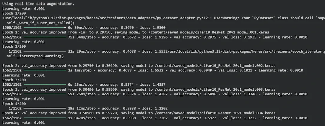
The model shows smooth convergence with increasing training accuracy, stable validation accuracy and decreasing losses. A small accuracy gap suggests mild overfitting but overall performance on CIFAR-10 is strong.

ResNet Results on ImageNet and COCO

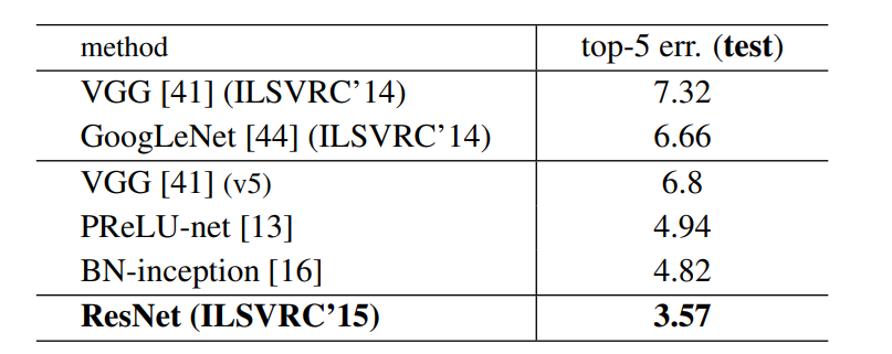
On the ImageNet dataset, the authors used a 152-layer ResNet, which is 8 times deeper than VGG-19 but still has fewer parameters. An ensemble of these ResNets achieved only 3.7% error on the ImageNet test set. On the COCO object detection dataset ResNet also produced a 28% relative improvement due to its very deep feature representation.

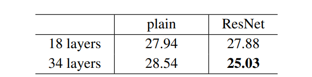
The results show that shortcut connections effectively address the problems caused by increasing network depth as increasing layers from 18 to 34 leads to a decrease in error rate on the ImageNet validation set unlike plain networks.

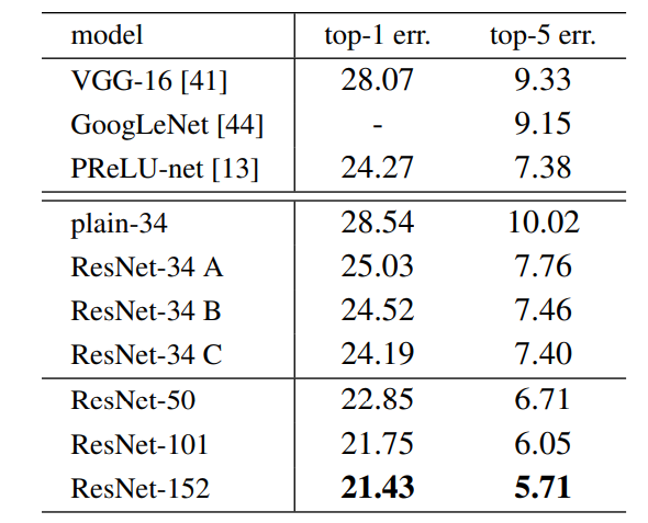
Below are the results on ImageNet Test Set. The 3.57% top-5 error rate of ResNet was the lowest and thus ResNet architecture came first in ImageNet classification challenge in 2015.

Advantages

• Eases Training of Deep Networks: Skip connections allow gradients to flow directly through the network, reducing vanishing gradient problems.
• Enables Very Deep Architectures: ResNet can train networks with 50, 100 or even 152+ layers effectively.
• Improves Accuracy: Residual learning helps the network achieve higher performance on tasks like image classification and object detection.
• Reduces Degradation: Adding more layers does not increase training error unlike plain deep networks.
• Fewer Parameters for Better Efficiency: Deep ResNets can have fewer parameters than traditional deep networks but performing better.

Challenges

• High Computation: Requires high computational power due to deep architecture.
• Dimension Mismatch: Dimension mismatch in skip connections needs extra projection layers.
• Overfitting Risk: Risk of overfitting on small datasets because of large model capacity.
• Training Instability: Training can become unstable without proper batch normalization.
• Redundant Updates: Residual blocks may learn only small or redundant updates.
• Deep Network Degradation: Gradient flow improves but may still degrade in extremely deep networks.