Categorical Cross-Entropy Loss in Multi-Class Classification: Complete Guide with Formula & Examples

Categorical Cross-Entropy is widely used as a loss function to measure how well a model predicts the correct class in multi-class classification problems. It measures the difference between the predicted probability distribution and the true one-hot encoded labels, guiding the model to assign higher probabilities to the correct class.

• It is used when there are more than two classes.
• Works with softmax outputs where probabilities sum to 1.
• Higher loss means the prediction is far from the true class, lower loss means the model is performing well.
• Commonly used in image classification, text classification and speech recognition tasks.

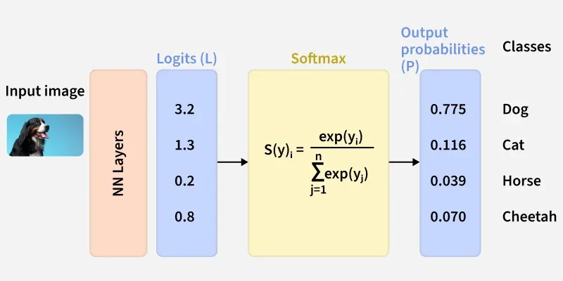
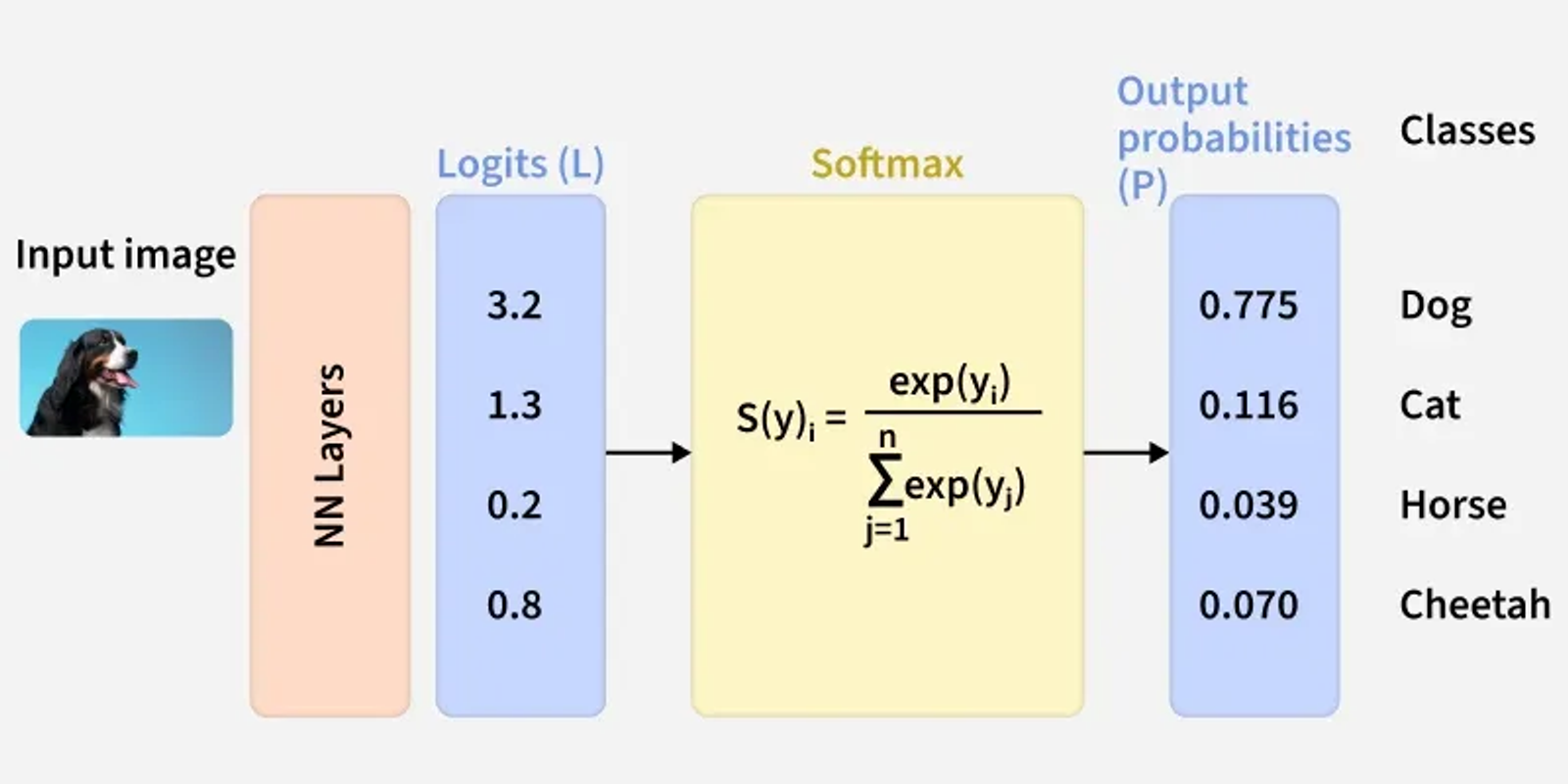
Here we see how neural networks are converted into Softmax probabilities and used in Categorical Cross-Entropy (CCE) to compute loss for the true class.

How Categorical Cross-Entropy Works

Categorical Cross-Entropy measures the difference between the true labels and the predicted probabilities of a model. It penalizes the model when it assigns low confidence to the correct class. Formula is:

where

• [@portabletext/react] Unknown block type "latex", specify a component for it in the `components.types` prop: Categorical Cross-Entropy loss
• [@portabletext/react] Unknown block type "latex", specify a component for it in the `components.types` prop: True label for class ii
• [@portabletext/react] Unknown block type "latex", specify a component for it in the `components.types` prop: Predicted probability for class ii
• C: Number of classes

Categorical Cross-Entropy works through the following steps

• Prediction of Probabilities: The model uses a Softmax layer to convert raw logits into probabilities for each class.
• Comparison with True Class: Predicted probabilities are matched with one-hot encoded labels to determine the correct class.
• Calculation of Loss: CCE calculates the negative log of the predicted probability for the true class, giving lower loss for higher confidence and higher penalty for low confidence.

Step-By-Step Implementation

Here in this code we will train a neural network on the MNIST dataset using Categorical Cross-Entropy loss for multi-class classification. It allows predicting any test image and displays the probability of each class along with the predicted label.

Step 1: Import Libraries & Load Dataset

Here we will use numpy, tensorflow and matplotlib

import numpy as np
import tensorflow as tf
from tensorflow.keras.datasets import mnist
from tensorflow.keras.models import Sequential
from tensorflow.keras.layers import Dense, Flatten
from tensorflow.keras.utils import to_categorical
from tensorflow.keras.losses import CategoricalCrossentropy
import matplotlib.pyplot as plt

(X_train, y_train), (X_test, y_test) = mnist.load_data()

Step 2: Preprocess Data

• Normalization: Scale pixel values to [0,1] for faster training
• One-hot encoding: Convert integer labels to categorical format
• Categorical labels: Required for multi-class classification

X_train = X_train.astype('float32') / 255.0
X_test = X_test.astype('float32') / 255.0
y_train_encoded = to_categorical(y_train, num_classes=10)
y_test_encoded = to_categorical(y_test, num_classes=10)

Step 3: Build and Compile Model

• Use a Sequential model with Dense layers and ReLU activation
• Flatten input images before feeding into Dense layers.
• Use Softmax activation in output layer for 10 classes.
• Compile the model with Adam optimizer and Categorical Cross-Entropy (CCE) loss.

model = Sequential([
    Flatten(input_shape=(28,28)),
    Dense(128, activation='relu'),
    Dense(64, activation='relu'),
    Dense(10, activation='softmax') 
])

model.compile(optimizer='adam',
              loss=CategoricalCrossentropy(),
              metrics=['accuracy'])

Step 4: Train the Model

• Epoch: One complete pass over the training data
• Batch size: Number of samples per gradient update
• Validation split: 20% of training data used to check model performance
• Categorical Crossentropy (CCE) loss: Guides the model to improve predictions
• Training loss and accuracy: Metrics to monitor learning progress

history = model.fit(X_train, y_train_encoded, epochs=10, batch_size=64, validation_split=0.2)

Step 5: Predict and Display Probabilities

• Softmax probabilities: Model outputs probability distribution over classes
• Predicted class: Class with highest probability
• Visualization: Display the test image and prediction
• Categorical Cross-Entropy: Loss used during training

def predict_digit(index):
    img = X_test[index]
    plt.imshow(img, cmap='gray')
    plt.title(f"True Label: {y_test[index]}")
    plt.axis('off')
    plt.show()
    
    pred_prob = model.predict(img.reshape(1,28,28))[0]
    for i, prob in enumerate(pred_prob):
        print(f"Class {i}: {prob:.4f}")
    predicted_class = np.argmax(pred_prob)
    print(f"\nPredicted Class: {predicted_class}")

Categorical Cross-Entropy vs Binary Cross-Entropy

Here we see the difference between Categorical Cross-Entropy and Binary Cross-Entropy

Applications

• Handwritten Digit Recognition: Classifying digits 0 to 9 in apps like postal mail sorting.
• Email Classification: Categorizing emails into multiple folders like Inbox, Promotions Social, etc.
• Sentiment Analysis: Determining if a review is Positive, Negative or Neutral.
• Medical Imaging: Detecting types of diseases from X-rays or MRI scans.
• Speech Recognition: Recognizing different words or commands in voice assistants.

Advantages

• Effective for Multi-Class Problems: Perfectly suited for tasks with more than two classes.
• Probabilistic Interpretation: Works naturally with Softmax outputs to produce meaningful probabilities.
• Sensitive to Incorrect Predictions: Penalizes wrong predictions more helping models learn better.
• Smooth Gradient: Provides continuous and differentiable loss ideal for gradient-based optimization.

Limitations

• Requires One-Hot Labels: Needs proper encoding of true labels, not suitable for raw class integers.
• Overconfidence Risk: Models can become overconfident in predictions if not regularized.
• Not for Multi-Label Problems: Works for single-class predictions per sample, not multi-label classification.
• Sensitive to Class Imbalance: Can give biased training if classes are unevenly distributed.