AlexNet Explained: The CNN That Revolutionized Deep Learning in 2012

AlexNet is a deep learning model that made a big impact in image recognition. It became famous for its ability to classify images accurately. It won the ImageNet Large Scale Visual Recognition Challenge (ILSVRC) 2012 with a top-5 error rate of 15.3% (beating the runner up which had a top5 error rate of 26.2%)

Most important features of the AlexNet are:

• Overfitting Prevention: Dropout (0.5) was applied to the first two fully connected layers and data augmentation dynamically expanded the dataset hence both helping in reducing overfitting.
• Faster Training: ReLU activation was used instead of tanh or sigmoid, leading to a 6x speedup in training by avoiding.

AlexNet Architecture

Its architecture includes:

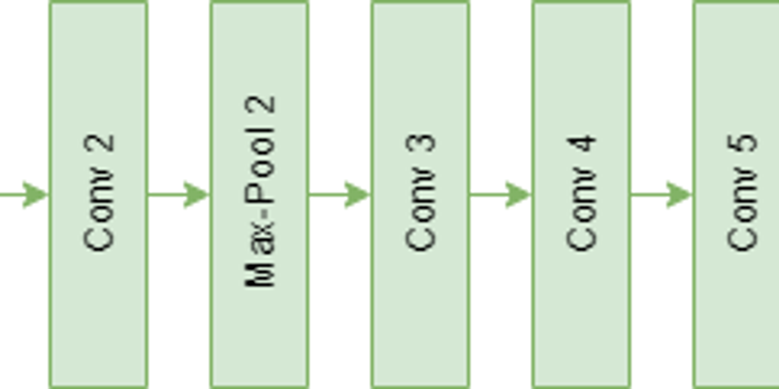
• 5 convolutional layers with Max-Pooling applied after the 1st, 2nd and 5th layers to enhance feature extraction.
• Overlapping Max-Pooling uses a 3×3 filter with stride 2 which improved performance by reducing top-1 error by 0.4% and top-5 error by 0.3% compared to non-overlapping pooling.
• Followed by 2 fully connected layers each using dropout to prevent overfitting.
• Ends with a softmax layer for final classification.

Implementation of AlexNet for Object Classification

Here we will see step by step implementation of alexnet model:

1. Import Libraries

We import tensorflow and matplotlib for it.

import tensorflow as tf
from tensorflow.keras.models import Sequential
from tensorflow.keras.layers import Conv2D, MaxPooling2D, Flatten, Dense, Activation, Dropout, BatchNormalization
from tensorflow.keras.datasets import cifar10
from tensorflow.keras.utils import to_categorical
import matplotlib.pyplot as plt

2. Load and Preprocess CIFAR-10 Dataset

• CIFAR-10 contains 60.000x32x32 RGB images across 10 classes.
• Pixel values are scaled to [0,1].
• Labels are one-hot encoded for softmax classification

# Load CIFAR-10 data
(x_train, y_train), (x_test, y_test) = cifar10.load_data()

# Normalize pixel values
x_train = x_train.astype('float32') / 255.0
x_test = x_test.astype('float32') / 255.0

# One-hot encode the labels
y_train = to_categorical(y_train, 10)
y_test = to_categorical(y_test, 10)

3. Define the AlexNet Model (Adjusted for CIFAR-10)

• Adjusted to CIFAR-10's 32×32 input size and 10 output classes.
• Reduced FC layers from 4096→1024→512 to avoid overfitting on small images.
• Uses ReLU, Dropout, BatchNorm and softmax in the final layer.

model = Sequential()

# Layer 1
model.add(Conv2D(96, kernel_size=(3,3), strides=(1,1), input_shape=(32,32,3), padding='same'))
model.add(Activation('relu'))
model.add(MaxPooling2D(pool_size=(2,2), strides=(2,2)))
model.add(BatchNormalization())

# Layer 2
model.add(Conv2D(256, kernel_size=(3,3), strides=(1,1), padding='same'))
model.add(Activation('relu'))
model.add(MaxPooling2D(pool_size=(2,2), strides=(2,2)))
model.add(BatchNormalization())

# Layer 3
model.add(Conv2D(384, kernel_size=(3,3), strides=(1,1), padding='same'))
model.add(Activation('relu'))

# Layer 4
model.add(Conv2D(384, kernel_size=(3,3), strides=(1,1), padding='same'))
model.add(Activation('relu'))

# Layer 5
model.add(Conv2D(256, kernel_size=(3,3), strides=(1,1), padding='same'))
model.add(Activation('relu'))
model.add(MaxPooling2D(pool_size=(2,2), strides=(2,2)))

# Flatten
model.add(Flatten())

# Fully Connected Layer 1
model.add(Dense(1024))
model.add(Activation('relu'))
model.add(Dropout(0.5))

# Fully Connected Layer 2
model.add(Dense(512))
model.add(Activation('relu'))
model.add(Dropout(0.5))

# Output Layer
model.add(Dense(10))
model.add(Activation('softmax'))

4. Compile the Model

We use adam optimizer and categorical_crossentropy for multi-class classification.

model.compile(loss='categorical_crossentropy',
              optimizer='adam',
              metrics=['accuracy'])

5. Train the Model

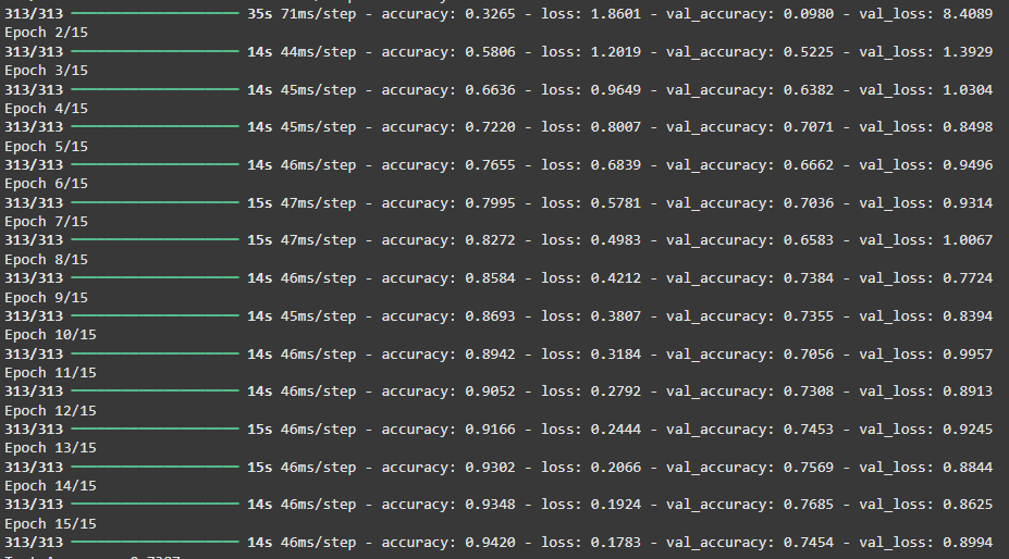
• Train for 15 epochs, with 20% validation split.
• You can increase epochs for better accuracy.

history = model.fit(x_train, y_train,
                    batch_size=128,
                    epochs=15,
                    validation_split=0.2,
                    verbose=1)

Output:

6. Evaluate the Model

test_loss, test_acc = model.evaluate(x_test, y_test, verbose=0)
print(f'Test Accuracy: {test_acc:.4f}')

7. Plot Training & Validation Accuracy

plt.plot(history.history['accuracy'], label='Train Accuracy')
plt.plot(history.history['val_accuracy'], label='Validation Accuracy')
plt.title('AlexNet on CIFAR-10 (GPU)')
plt.xlabel('Epochs')
plt.ylabel('Accuracy')
plt.legend()
plt.grid(True)
plt.show()

Output:

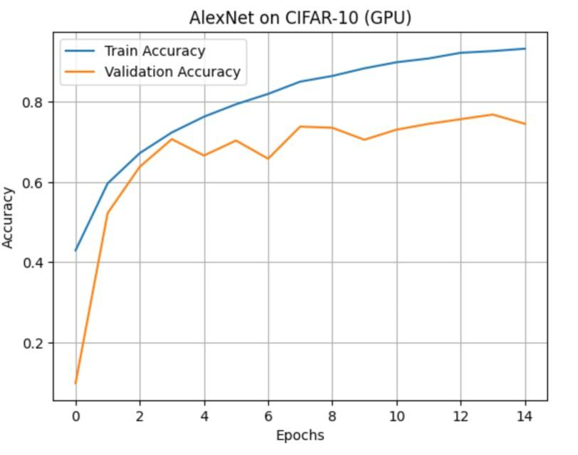
We can see that train and validation accuracy is quit similar in end meaning our model is working fine.

Advantages of AlexNet

• Use of ReLU Activation: First major architecture to use ReLU (Rectified Linear Unit) which enabled faster training compared to traditional tanh/sigmoid functions.
• Dropout for Regularization: Introduced dropout layers to reduce overfitting by randomly disabling neurons during training.
• GPU Utilization: Split the network across two GPUs, showing how deep learning can benefit from parallel computing for faster training.
• Overlapping Max-Pooling: Used overlapping pooling layers to improve generalization and reduce top-1 and top-5 classification errors.

Disadvantages of AlexNet

• Large Model Size: Has around 60 million parameters making it memory-intensive and slow for inference on low-resource devices.
• High Computational Cost: Training is computationally expensive even though it was optimized for GPUs.
• Manual Architecture Design: The architecture lacks modularity and automation, unlike modern approaches like NAS or EfficientNet.
• Not Optimal for Small Datasets: Tends to overfit on smaller datasets like CIFAR-10 or MNIST without heavy regularization.
• Outdated Compared to Modern Architectures: Lacks innovations like residual connections (ResNet), depthwise separable convolutions (MobileNet) and attention mechanisms (ViT).

Applications

1. Image Classification: Originally built for classifying high-resolution images into 1000 object categories (ImageNet dataset).
2. Feature Extraction: Intermediate layers are often used as pretrained feature extractors for transfer learning tasks.
3. Object Detection: Forms the backbone in early detection systems like R-CNN when combined with region proposal methods.
4. Medical Imaging: Applied to classify abnormalities in X-rays, MRIs or retinal scans by fine-tuning on domain-specific datasets.
5. Facial Recognition and Emotion Detection: Can be adapted for face verification, expression analysis or identity recognition tasks.
6. Autonomous Vehicles: Used in early perception modules for identifying road signs, pedestrians or obstacles.