Adagrad Optimizer in Deep Learning: How It Works & When to Use It

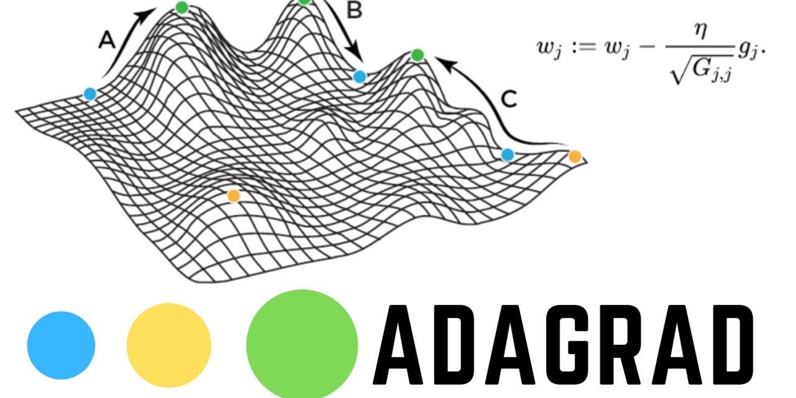
Adagrad (Adaptive Gradient Algorithm) is an optimization method that adjusts the learning rate for each parameter during training. Unlike standard gradient descent with fixed rate, Adagrad uses past gradients to scale updates making it effective for sparse data and varying features magnitudes.

Working Adagrad

The primary concept behind Adagrad is the idea of adapting the learning rate based on the historical sum of squared gradients for each parameter. Here;s a step-by-step explanation of how Adagrad works:

1. Initialization: Adagrad begins by initializing the parameter values randomly, just like other optimization algorithms. Additionally, it initializes a running sum of squared gradients for each parameter which will track the gradients over item.
2. Gradient Calculation: For each training step, the gradient of the loss function with respect to the model’s parameters is calculated, just like in standard gradient descent.
3. Adaptive Learning Rate: The key difference comes next. Instead of using a fixed learning rate, Adagrad adjusts the learning rate for each parameter based on the accumulated sum of squared gradients.

The updated learning rate for each parameter is calculated as follows:

Where:

• η is the global learning rate (a small constant value)
• Gt is the sum of squared gradients for a given parameter up to time step t
• ϵ is a small value added to avoid division by zero (often set to 1e−8)

4. Parameter Update: The model's parameters are updated by subtracting the product of the adaptive learning rate and the gradient at each step:

When to Use Adagrad?

Adagrad is ideal for:

• Problems with sparse data and features like in natural language processing or recommender systems.
• Tasks where features have different levels of importance and frequency
• Training models that do not require a very fast convergence rate but benefit from more stable optimization process.

However, if you are dealing with problems where a more constant learning rate is preferable, using variants like RMSProp or Adam might be more appropriate

Different Variants of Adagrad Optimizer

To address some of Adagrad’s drawbacks, a few improved versions have been created like:

1. RMSProp (Root Mean Square Propagation):

RMSProp addresses the diminishing learning rate issue by introducing an exponentially decaying average of the squared gradients instead of accumulating the sum. This prevents the learning rate from decreasing too quickly, making the algorithm more effective in training deep neural networks.

The update rule for RMSProp is as follows:

Where:

• [@portabletext/react] Unknown block type "latex", specify a component for it in the `components.types` prop​ is the accumulated gradient
• γ is the decay factor (typically set to 0.9)
• [@portabletext/react] Unknown block type "latex", specify a component for it in the `components.types` prop is the gradient

The parameter update rule is:

2. AdaDelta

AdaDelta is another modification of Adagrad that focuses on reducing the accumulation of past gradients. It updates the learning rates based on the moving average of past gradients and incorporates a more stable and bounded update rule.

The key update for AdaDelta is:

Where:

• [@portabletext/react] Unknown block type "latex", specify a component for it in the `components.types` propis the running average of past squared parameter updates

3. Adam (Adaptive Moment Estimation)

Adam combines the benefits of both Adagrad and momentum-based methods. It uses both the moving average of the gradients and the squared gradients to adapt the learning rate. Adam is widely used due to its robustness and superior performance in various machine learning tasks.

Adam has the following update rules:

• First moment estimate ([@portabletext/react] Unknown block type "latex", specify a component for it in the `components.types` prop):

• Second moment estimate ([@portabletext/react] Unknown block type "latex", specify a component for it in the `components.types` prop):

• Corrected moment estimates:

• Parameter update:

Adagrad Optimizer Implementation

Below are examples of how to implement the Adagrad optimizer in TensorFlow and PyTorch.

1. TensorFlow Implementation

In TensorFlow, implementing Adagrad is easier as it’s already includes in the API. Here’s an example where:

• mnist.load_data() loads the MNIST dataset.
• reshape() flattens 28x28 images into 784-length vectors.
• Division by 255 normalizes pixel values to [0,1].
• tf.keras.Sequential() builds the neural network model.
• tf.keras.layers.Dense() creates fully connected layers.
• activation='relu' adds non-linearity in hidden layer and softmax outputs probabilities.
• tf.keras.optimizers.Adagrad() applies adaptive learning rates per parameter to improve convergence.
• compile() configures training with optimizer, loss function and metrics.
• loss='sparse_categorical_crossentropy' computes loss for integer class labels.
• model.fit() trains the model for specified epochs on the training data.

import tensorflow as tf
from tensorflow.keras.datasets import mnist
from tensorflow.keras.utils import to_categorical

(x_train, y_train), (x_test, y_test) = mnist.load_data()

x_train = x_train.reshape(-1, 784).astype('float32') / 255.0
x_test = x_test.reshape(-1, 784).astype('float32') / 255.0

model = tf.keras.Sequential([
    tf.keras.layers.Dense(64, activation='relu', input_shape=(784,)),
    tf.keras.layers.Dense(10, activation='softmax')
])

model.compile(optimizer=tf.keras.optimizers.Adagrad(learning_rate=0.01),
              loss='sparse_categorical_crossentropy',
              metrics=['accuracy'])

model.fit(x_train, y_train, epochs=5)

2. PyTorch Implementation

In PyTorch, Adagrad can be used with the torch.optim.Adagrad class. Here's an example where:

• datasets.MNIST() loads data, ToTensor() converts images and Lambda() flattens them.
• DataLoader batches and shuffles data.
• SimpleModel has two linear layers with ReLU in forward().
• CrossEntropyLoss computes classification loss.
• Adagrad optimizer adapts learning rates per parameter based on past gradients, improving training on sparse or noisy data.
• Training loop: zero gradients, forward pass, compute loss, backpropagate and update weights with Adagrad.

import torch
import torch.nn as nn
import torch.optim as optim
from torchvision import datasets, transforms
from torch.utils.data import DataLoader

transform = transforms.Compose([
    transforms.ToTensor(),
    transforms.Lambda(lambda x: x.view(-1))
])

train_dataset = datasets.MNIST(
    root='./data', train=True, download=True, transform=transform)
train_loader = DataLoader(train_dataset, batch_size=64, shuffle=True)


class SimpleModel(nn.Module):
    def __init__(self):
        super(SimpleModel, self).__init__()
        self.fc1 = nn.Linear(784, 64)
        self.fc2 = nn.Linear(64, 10)

    def forward(self, x):
        x = torch.relu(self.fc1(x))
        return self.fc2(x)


model = SimpleModel()

loss_fn = nn.CrossEntropyLoss()
optimizer = optim.Adagrad(model.parameters(), lr=0.01)

for epoch in range(5):
    for data, target in train_loader:
        optimizer.zero_grad()
        output = model(data)
        loss = loss_fn(output, target)
        loss.backward()
        optimizer.step()
    print(f"Epoch {epoch+1} complete")

By applying Adagrad in appropriate scenarios and complementing it with other techniques like RMSProp and Adam, practitioners can achieve faster convergence and improved model performance.

Advantages

• Adapts learning rates for each parameter, helping with sparse features and noisy data.
• Works well with sparse data by giving rare but important features appropriate updates.
• Automatically adjusts learning rates, eliminating the need for manual tuning.
• Improves performance in cases with varying gradient magnitudes, enabling efficient convergence.

Limitations

• Learning rates shrink continuously during training which can slow convergence and cause early stopping.
• Performance depends heavily on the initial learning rate choice.
• Lacks momentum, making it harder to escape shallow local minima.
• Learning rates decrease as gradients accumulate which helps avoid overshooting but may hinder progress later in training.